Analysis of coverage in capture experiments (v.4)
Merly Escalona merlyescalona@uvigo.es
Introduction
In order to integrate a new feature of on/off target levels of coverage in NGSphy, I needed to understand coverage variation that one could find in a capture experiment. Goals are basically:
- Understand the coverage variation within individuals and loci to be able to model it for both NGSphy parameterization and furthers simulations.
- Find out whether there is a correlation between the coverage and the phylogenetic distance to the reference species that were used for the probe generation. Expecting that the closer the sample is to the reference the higher the coverage obtained is.
Data description
General
- Reference genomes: Reference genomes for Calypte anna [1] and Chaetura pelagica [2] are available. As well as the codon regions per species (
Calypte_anna.gene.CDS.gffandChaetura_pelagica.CDS.gff)
Genome sizes
| Anna | Swift |
|---|---|
| 1,114,626,264 | 1,125,117,173 |
- One-to-one orthologs: There is information available about the one-to-one ortholog relation between the species from the Avian Genome Consortium . (
48birds_ortholog.list.chi.anna.cpe.hum.finch).
Hummingbirds paper
Data used comes from Rute’s Hummingbird project. Most of the information reported here about the samples and targets was extracted from the paper.
- Samples: species were chosen so that all the nine major Trochiliform clades reported by Bleiweiss et al. [3] and McGuire et al. [4] and many of the characteristic subclades illustrated by McGuire et al. [2] were represented.
- 32 species - the National Museum of Natural History, Smithsonian Institution
- 14 species - the Louisiana State University Museum of Natural Sciences
- Target regions: probes were selected from one-to-one orthologs between chicken (Gallus gallus) and zebra finch (Taeniopygia guttata) as annotated in ENSEMBL version 66 annotation resulting in a final set:
- 166.322 probes
- corresponding to 2950 genes
- summing up to approximately 20 Mb (for an approximately 7 Mb of total captured sequence).
- final analysis was made with 2750 genes, left after removing genes with missing data.
- The datasets I’m using
BAMfiles corresponding to the mappings of the targeted-sequencing to 2 references.- 46 files, corresponding to the samples mapped to an ingroup Calypte anna (from now on called
map2Anna).- 46 samples - targeted sequencing
- 48 files, corresponding to the samples an outgroup Chaetura pelagica (from now on called
map2Swift).- 46 samples - targeted sequencing
- 2 samples - whole genome sequencing (Anna + Swift)
- 46 files, corresponding to the samples mapped to an ingroup Calypte anna (from now on called
Missing data
Need more information on missing data id + removal
Processing and storage
Workspace triploid (UVigo):
- Original data from Dataset 1, is stored in:
triploid.uvigo.es - Under the user folder:
/home/merly/research/cph-visit/coverage-analysis
Workspace randy (KU):
- Original data from Dataset 1 and 2, is stored in:
randy.popgen.dk - Under the user folder:
/home/merly/anna/home/merly/swift
Targeted regions
Targeted regions are exons, retrieved a posteriori, due to the fact that the original probes for this project were lost during a flood.
Ingroup species reference: Original target file given was a GFF file:Calypte_anna.gene.CDS.2750.gff[1.6MB]. This contains the exons from the 2,750 This file was converted into a BED file, keeping only chromosome (scaffold), start and end position of the targets.- Filtering regions with size 0
Outgroup reference:: For this one, I received 2 files. One that had the known one-to-one ortholog relation between the genes from Anna and Swift (48birds_ortholog.list.chi.anna.cpe.hum.finch[656KB]). The second, is a GFF file, which contains the exons from Swift (Chaetura_pelagica.CDS.gff[8.5MB]). I had to get the targeted regions from the GFF files, taking into account that I needed the genes matching to Anna, and also I needed those genes that were actually used in the Anna’s targets (Calypte_anna.gene.CDS.2750.gff):- Keep the gene that matched both Anna and Swift species within this file
48birds_ortholog.list.chi.anna.cpe.hum.finch. - Filter out those where there was no match (Gene in Anna == “-” or Gene in Swift == “-”)
- Filtering regions with size 0
- Check that all the targets in
Chaetura_pelagica.CDS.gffwhere codon regions (CDS). - Match the genes obtained in (4), to the data in
Calypte_anna.gene.CDS.2750.gffso I’ll have the same covered genes. - Match the resulting genes from (5) to
Chaetura_pelagica.CDS.gffand keep those targets from genes matching both Anna and Swift.
- Keep the gene that matched both Anna and Swift species within this file
Finally, datasets will be filter to match gene number.
birds48filename=paste0(WD,"48birds_ortholog.list.chi.anna.cpe.hum.finch")
swiftgff=paste0(WD,"Chaetura_pelagica.CDS.gff")
annagff=paste0(WD,"Calypte_anna.gene.CDS.2750.gff")
birds=read.table(birds48filename, header=T,
colClasses=c("character","numeric","character","character",
"character","character","character"))
swift=read.table(swiftgff,
colClasses=c("character","character","character","numeric",
"numeric","character","character","character","character"))
anna=read.table(annagff,
colClasses=c("character","character","character","numeric",
"numeric","character","character","character","character"))
birds.2=birds[birds$anna!="-",]
birds.3=birds.2[birds.2$swift!="-",]
birds.4=unique(birds.3)
birds.5=birds.4[,c("anna","swift")]
birds.5$swift=paste0("Parent=",birds.5$swift,";")
birds.5$anna=paste0("Parent=Aan_", birds.5$anna,";")
annaGenes=unique(anna$V9[birds.5$anna %in% anna$V9])
birds.6=birds.5[birds.5$anna %in% annaGenes, ]
swiftGenes=birds.6$swift
swift.2=swift[swift$V3=="CDS",]
swift.3=swift.2[swift.2$V9 %in% birds.6$swift,]
swift.3$size=swift.3$V5-swift.3$V4
swift.4=swift.3[swift.3$size>0,]
anna.2=anna[(anna$V5-anna$V4)>0,]
swift.4=swift.4[,1:(ncol(swift.4)-1)]
anna.3=anna.2[anna.2$V9 %in% unique(birds.6$anna),]
anna.3$targetname=paste0( anna.3$V1,
rep("-", nrow(anna.3)),
anna.3$V4,
rep("-", nrow(anna.3)),
anna.3$V5)
swift.4$targetname=paste0( swift.4$V1,
rep("-", nrow(swift.4)),
swift.4$V4,
rep("-", nrow(swift.4)),
swift.4$V5)Description of the targeted regions
This is a quantitative summary description of the resulting target files. The difference between number of genes, and subsequently in number of targets and covered genome, in both Anna and Swift, is not precisely alarming. The experiment was done using known ortholog genes, which not necessarily match in number of exons (targets) or their size. There are two (2) Anna datasets, the original and the reduced (1,469 genes) and the Swift dataset.
| Number of targets | Size of targeted genome (bp) | Number of genes | Total of scaffolds | |
|---|---|---|---|---|
| Anna - Original | 24,044 | 3,934,867 | 2,750 | 389 |
| Anna - Reduced | 14,740 | 2,285,746 | 1,469 | 314 |
| Swift | 14,764 | 2,279,626 | 1,469 | 372 |
SARA COMMENT
- So, the size of the “targeted genome” in both Anna and Swift is ~3.9Mb and ~2.2Mb… that’s quite a difference from the “rough” reported 7M in the paper … [just a comment…]
Number of targeted regions per gene

Number of targeted regions per scaffold
- Scaffolds: where genes are located.

Gene size distribution

| Min. | 1st Qu. | Median | Mean | 3rd Qu. | Max. | |
|---|---|---|---|---|---|---|
| Anna - Original | 104 | 724 | 1,136 | 1,431 | 1,800 | 13,150 |
| Anna - Reduced | 110 | 842 | 1,285 | 1,556 | 1,953 | 13,150 |
| Swift | 110 | 843 | 1,281 | 1,552 | 1,943 | 13,000 |
Targeted regions size distribution

| Min. | 1st Qu. | Median | Mean | 3rd Qu. | Max. | |
|---|---|---|---|---|---|---|
| Anna - Original | 1 | 90 | 125 | 163.7 | 170 | 5,246 |
| Anna - Reduced | 1 | 90 | 125 | 163.2 | 169 | 5,246 |
| Swift | 1 | 89 | 123 | 154.4 | 166 | 5,240 |
- These target size distribution are pretty much alike, but, there are some targeted regions up to ~5Kb. A question that can appear is whether these regions were expected (in terms of size). The idea with this experiment was to capture whole genes, and for this reason, theses sizes are not unexpected. Depth of coverage, which is what is being analyze here, depends more on probe feature decisions like size and density of the tiling.
SARA COMMENT
‘> 5kb’ fragments? ok, “idea was to capture whole genes” but “targets” are CONTIGUOUS regions, right? pretty much like our loci, right? Were probes designed from fragments > 5kb? hard to believe…
On-target coverage
NOTE
Target datasets used from now on will contain the same number of genes (1,469).
I obtained the coverage of the targeted regions using bedtools[9] (v. 2.22.0), module coverage. With this, and the option -hist I can report a histogram of coverage for each feature in A as well as a summary histogram for _all_ features in A. Output (tab delimited) after each feature in A (from bedtools documentation))
- depth
#bases at depth- size of A
- % of A at depth
for bamfile in $(find $HOME/anna/originals -name "*.bam"); do
tag=$(echo $(basename $bamfile) | tr "_" " " | awk '{print $1}')
nohup bedtools coverage -hist -abam $bamfile -b "Calypte_anna.gene.CDS.2750.3.gff" | gzip > $HOME/anna/bedtools/cov/${tag}.cov.gz &
done
for bamfile in $(find $HOME/swift/originals -name "*.bam"); do
tag=$(echo $(basename $bamfile) | tr "_" " " | awk '{print $1}')
nohup bedtools coverage -hist -abam $bamfile -b "Chaetura_pelagica.CDS.2.gff" | gzip > $HOME/swift/bedtools/cov/${tag}.cov.gz &
doneAnd so, I filtered the output to keep the coverage per region and the summary histogram separated.
# (i.e)
for tag in $(cat $HOME/anna/files/samples.txt ); do
nohup zcat $HOME/anna/bedtools/cov/H09.cov.gz | grep -v ^all | gzip > $HOME/anna/bedtools/nohist/$tag.nohist.gz &
nohup zcat $HOME/anna/bedtools/cov/H09.cov.gz | grep ^all | gzip > $HOME/anna/bedtools/hist/$tag.hist.gz &
done
for tag in $(cat $HOME/swift/files/samples.txt | tail -n+2 | head -46 ); do
nohup zcat $HOME/swift/bedtools/cov/H09.cov.gz | grep -v ^all | gzip > $HOME/swift/bedtools/nohist/$tag.nohist.gz &
nohup zcat $HOME/swift/bedtools/cov/H09.cov.gz | grep ^all | gzip > $HOME/swift/bedtools/hist/$tag.hist.gz &
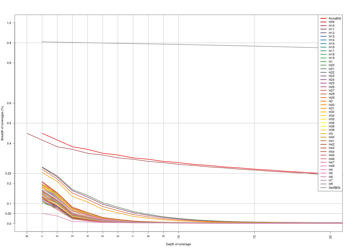
doneBreadth vs. depth
With the information extracted from the bedtools coverage -hist, we can see the relation between the breadth of coverage obtained and the depth per sample. This gives the fraction of the captured genome against the coverage.
| Map2 - target | Coverage per target overview |
|---|---|
| map2Anna | 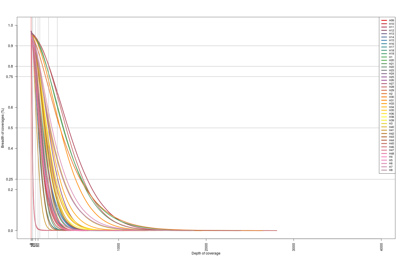 |
| map2Swift | |
(Click image to enlarge)
Zoom: 0x-100x.
| map2Anna | map2Swift |
|---|---|
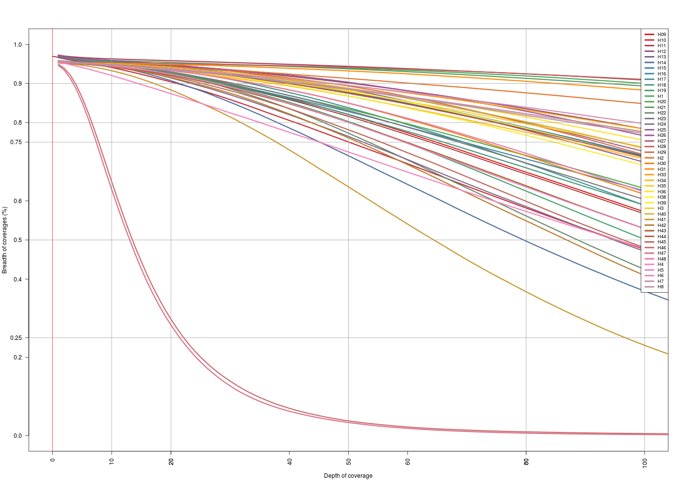 |
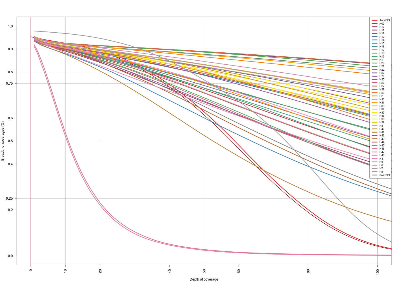 |
(Click image to enlarge)
SARA COMMENT
On the depth vs breath… the zoom 0x-100x… is it OK? Is the scale the same? It does not look like…
- Then its PER TARGET, but there are no targets > 5kb… excluded or w/ very very low depth of coverage (in a big portion of it)
Outlier calculations
Outliers presented in this report were calculated using the following:
qnt <- quantile(data, probs=c(.25, .75))
H <- 1.5 * IQR(data)
y <- data
y[data < (qnt[1] - H)] <- "Outlier"
y[data > (qnt[2] + H)] <- "Outlier"Depth of coverage
From the bedtools coverage output I was able to extract the depth of coverage per target, gene and sample.
I generated 2 matrices:
- Target depth: dimensions – number of targets \(\times\) number of samples
- Gene depth: dimensions – number of genes \(\times\) number of samples
Each cell of the matrix correspond to the sum of the number of times each base was covered within the target or the gene. Then, coverage was calculated as the mean value of all the depth of coverage of all the samples for a specific target/gene divided by the size of the corresponding target/gene.
For the depth of coverage for the samples, I summed the coverage of all targets and divided it by the total amount of bases that were targeted.
Related to the language
Everything is just average depth of coverage (individual/gene and target)
Coverage per sample
Depth per sample

Coverage distribution per sample

| Min. | 1st. Qu. | Median | Mean | 3rd. Qu | Max. | Var. | Std. Dev | |
|---|---|---|---|---|---|---|---|---|
| map2Anna | 2.115 | 47.76 | 77.73 | 101.3 | 115.8 | 310.2 | 6,616.195 | 81.34 |
| map2Swift | 1.715 | 38.27 | 62.29 | 83.8 | 98.07 | 265.6 | 4,931.13 | 70.22201 |
| map2Anna without outliers | 2.115 | 44.22 | 64.82 | 74.42 | 93.6 | 177.6 | 1,886.191 | 43.4303 |
| map2Swift without outliers | 1.715 | 35.94 | 50.84 | 61.49 | 76.74 | 156.5 | 1,530.202 | 39.1178 |
Coverage per gene

| Min. | 1st. Qu. | Median | Mean | 3rd. Qu | Max. | Var. | Std. Dev | |
|---|---|---|---|---|---|---|---|---|
| map2Anna | 12.05 | 72.38 | 98.38 | 105 | 133.5 | 290.3 | 2,134.744 | 46.2033 |
| map2Swift | 0.8245 | 54.24 | 81.06 | 85.55 | 111.5 | 702.6 | 2,039.718 | 45.16324 |
Outlier check - map2Anna
Identification and removal of the outliers
- Details of the gene with extremely high coverage.
- First, there is a table with the details of the gene, specific targets (exon regions, size and coverage)
- IGV Capture of the region, where it is possible to see several peaks, more that the number of targets for this region, with high coverage.
- There is also a zoomed region, belonging to the
scaffold116, positions5,306,081-5,306,303.AShows the coverage distribution, as plotted by IGV. While,B, shows the bottom of the region coverage peak, and the corresponding nucleotide sequence. - It might be possible that this is a repetitive element, and so, the reason why it has so high coverage.
extHighCoverageGene=coveragePerGeneSwift[outliersSwift>0]
extHighCoverageGene=extHighCoverageGene[extHighCoverageGene>300]
# Cpe_R001479
swiftSplitGene=split(swift.4,swift.4$V9)
dd=swiftSplitGene[names(extHighCoverageGene)][[1]]
dd$Size=dd$V5-dd$V4
dd=dd[c(1,4,5,9,11)]
colnames(dd)=c("Scaffold","Start", "End","Gene name","Size")
kable(dd, format="markdown", row.names = F)| Scaffold | Start | End | Gene name | Size |
|---|---|---|---|---|
| scaffold116 | 5296564 | 5296613 | Parent=Cpe_R001479; | 49 |
| scaffold116 | 5301761 | 5301875 | Parent=Cpe_R001479; | 114 |
| scaffold116 | 5302539 | 5302571 | Parent=Cpe_R001479; | 32 |
| scaffold116 | 5305161 | 5305355 | Parent=Cpe_R001479; | 194 |
| scaffold116 | 5306081 | 5306303 | Parent=Cpe_R001479; | 222 |
| scaffold116 | 5308066 | 5308165 | Parent=Cpe_R001479; | 99 |
| scaffold116 | 5316336 | 5316420 | Parent=Cpe_R001479; | 84 |
 (Click image to enlarge)
(Click image to enlarge)
 (Click image to enlarge)
- Number of outliers genes and coverage distribution
| Num. outliers | Min. | 1st. Qu. | Median | Mean | 3rd. Qu. | Max. | |
|---|---|---|---|---|---|---|---|
| map2Anna | 21 | 225.2 | 237.3 | 251.2 | 255.5 | 272.8 | 290.3 |
| map2Swift | 19 | 199.1 | 207.3 | 215.7 | 246.4 | 234.3 | 702.6 |
- Outlier genes and corresponding size
| map2Anna Gene | map2Anna Size | map2Swift Gene | map2Size Gene |
|---|---|---|---|
| Parent=Aan_R000557; | 1025 | Parent=Cpe_R000257; | 1008 |
| Parent=Aan_R000645; | 1400 | Parent=Cpe_R001479; | 794 |
| Parent=Aan_R000757; | 1675 | Parent=Cpe_R001695; | 145 |
| Parent=Aan_R000784; | 1089 | Parent=Cpe_R002655; | 431 |
| Parent=Aan_R000837; | 2118 | Parent=Cpe_R003268; | 137 |
| Parent=Aan_R001079; | 884 | Parent=Cpe_R003836; | 461 |
| Parent=Aan_R001728; | 598 | Parent=Cpe_R004636; | 640 |
| Parent=Aan_R001861; | 604 | Parent=Cpe_R005332; | 1643 |
| Parent=Aan_R001895; | 3276 | Parent=Cpe_R008000; | 282 |
| Parent=Aan_R002476; | 896 | Parent=Cpe_R008889; | 709 |
| Parent=Aan_R003858; | 992 | Parent=Cpe_R011470; | 349 |
| Parent=Aan_R004237; | 3287 | Parent=Cpe_R012383; | 1214 |
| Parent=Aan_R004624; | 801 | Parent=Cpe_R012980; | 925 |
| Parent=Aan_R005273; | 508 | Parent=Cpe_R013031; | 753 |
| Parent=Aan_R005275; | 340 | Parent=Cpe_R013115; | 774 |
| Parent=Aan_R006006; | 360 | Parent=Cpe_R013182; | 2619 |
| Parent=Aan_R006018; | 584 | Parent=Cpe_R013834; | 743 |
| Parent=Aan_R006633; | 1151 | Parent=Cpe_R014755; | 608 |
| Parent=Aan_R007365; | 2134 | Parent=Cpe_R014832; | 1370 |
| Parent=Aan_R007414; | 1060 | ||
| Parent=Aan_R008340; | 964 |
- There is no correspondence of gene outliers across datasets:
- knownOrthologs[geneOutliersInAnna] \(\cap\) geneOutliersInSwift \(=\) \(\emptyset\)
Depth of coverage distribution per gene after removing outliers

| Min. | 1st. Qu. | Median | Mean | 3rd. Qu | Max. | Var. | Std. Dev | |
|---|---|---|---|---|---|---|---|---|
| map2Anna without outliers | 12.05 | 72.16 | 98.54 | 105 | 133.5 | 290.3 | 2,144.958 | 46.31369 |
| map2Swift without outliers | 0.8245 | 54.06 | 80.49 | 83.44 | 109.8 | 195.4 | 1,566.158 | 39.57471 |
Gene size vs. depth of coverage
I’m looking for a relation between gene size and depth of coverage. So I fit a linear model to the data.

lm() function that need to be discussed
##
## Call:
## lm(formula = coveragePerGeneAnnaFiltered ~ genesAnnaFiltered$Size)
##
## Residuals:
## Min 1Q Median 3Q Max
## -96.192 -32.445 -5.977 28.228 178.940
##
## Coefficients:
## Estimate Std. Error t value Pr(>|t|)
## (Intercept) 111.955749 2.051036 54.585 < 2e-16 ***
## genesAnnaFiltered$Size -0.004442 0.001065 -4.173 3.19e-05 ***
## ---
## Signif. codes: 0 '***' 0.001 '**' 0.01 '*' 0.05 '.' 0.1 ' ' 1
##
## Residual standard error: 46.05 on 1454 degrees of freedom
## Multiple R-squared: 0.01183, Adjusted R-squared: 0.01115
## F-statistic: 17.41 on 1 and 1454 DF, p-value: 3.19e-05
lm() function that need to be discussed
##
## Call:
## lm(formula = coveragePerGeneSwiftFiltered ~ genesSwiftFiltered$Size)
##
## Residuals:
## Min 1Q Median 3Q Max
## -83.810 -29.445 -2.706 26.272 111.522
##
## Coefficients:
## Estimate Std. Error t value Pr(>|t|)
## (Intercept) 84.8002830 1.7674363 47.979 <2e-16 ***
## genesSwiftFiltered$Size -0.0008706 0.0009156 -0.951 0.342
## ---
## Signif. codes: 0 '***' 0.001 '**' 0.01 '*' 0.05 '.' 0.1 ' ' 1
##
## Residual standard error: 39.58 on 1448 degrees of freedom
## Multiple R-squared: 0.000624, Adjusted R-squared: -6.614e-05
## F-statistic: 0.9042 on 1 and 1448 DF, p-value: 0.3418
Coverage per target

| Min. | 1st Qu. | Median | Mean | 3rd Qu. | Max. | |
|---|---|---|---|---|---|---|
| map2Anna | 0 | 34.12 | 84.28 | 167.6 | 178.3 | 42,890 |
| map2Swift | 0 | 23.04 | 64.59 | 136.6 | 144.9 | 56,610 |
Outliers check
- After the identification and removal of the outliers, this is number of target outliers and their coverage distribution
| Num. outliers | Min. | 1st. Qu. | Median | Mean | 3rd. Qu. | Max. | |
|---|---|---|---|---|---|---|---|
| map2Anna | 1,066 | 0 | 31.09 | 75.25 | 102 | 150 | 394.5 |
| map2Swift | 1,096 | 0 | 20.64 | 57.1 | 80.72 | 119.5 | 327.2 |
Depth of coverage distribution per target after removing coverage outliers

Size outliers removal
- Target size distribution: Target size distribution has not change since the beginning of the analysis, current size distribution can be shown here. For a proper finding of correlation between size and coverage I had to remove both, size outliers and coverage outliers.
Information of the depth coverage distribution of the outliers
| Num. outliers | Min. | 1st. Qu. | Median | Mean | 3rd. Qu. | Max. | |
|---|---|---|---|---|---|---|---|
| map2Anna | 810 | 0 | 34.75 | 80.78 | 106.3 | 155.3 | 394.5 |
| map2Swift | 814 | 0 | 23.12 | 60.83 | 84.11 | 124.2 | 327.2 |
Size distribution after removing outliers

| Min. | 1st. Qu. | Median | Mean | 3rd. Qu. | Max. | |
|---|---|---|---|---|---|---|
| map2Anna | 1 | 91 | 122 | 128.4 | 160 | 285 |
| map2Swift | 1 | 91 | 122 | 128.3 | 160 | 285 |
Coverage distribution after removing size and coverage related outliers

| Min. | 1st. Qu. | Median | Mean | 3rd. Qu | Max. | Var. | Std. Dev | |
|---|---|---|---|---|---|---|---|---|
| map2Anna without outliers | 0 | 34.75 | 80.78 | 106.3 | 155.3 | 394.5 | 8,395.816 | 91.62869 |
| map2Swift without outliers | 0 | 23.12 | 60.83 | 84.11 | 124.2 | 327.2 | 5,944.672 | 77.1017 |
Target size vs. depth of coverage
I’m looking for a relation between target size and depth of coverage.

lm() function that need to be discussed
##
## Call:
## lm(formula = anna.6$Coverage ~ anna.6$Size)
##
## Residuals:
## Min 1Q Median 3Q Max
## -167.95 -65.13 -20.57 47.08 337.69
##
## Coefficients:
## Estimate Std. Error t value Pr(>|t|)
## (Intercept) 168.43121 2.13600 78.85 <2e-16 ***
## anna.6$Size -0.48399 0.01548 -31.26 <2e-16 ***
## ---
## Signif. codes: 0 '***' 0.001 '**' 0.01 '*' 0.05 '.' 0.1 ' ' 1
##
## Residual standard error: 88.31 on 12742 degrees of freedom
## Multiple R-squared: 0.07122, Adjusted R-squared: 0.07115
## F-statistic: 977.1 on 1 and 12742 DF, p-value: < 2.2e-16
lm() function that need to be discussed
##
## Call:
## lm(formula = swift.7$Coverage ~ swift.7$Size)
##
## Residuals:
## Min 1Q Median 3Q Max
## -125.95 -56.29 -19.71 39.86 279.48
##
## Coefficients:
## Estimate Std. Error t value Pr(>|t|)
## (Intercept) 126.28067 1.81543 69.56 <2e-16 ***
## swift.7$Size -0.32870 0.01316 -24.98 <2e-16 ***
## ---
## Signif. codes: 0 '***' 0.001 '**' 0.01 '*' 0.05 '.' 0.1 ' ' 1
##
## Residual standard error: 75.28 on 12734 degrees of freedom
## Multiple R-squared: 0.0467, Adjusted R-squared: 0.04663
## F-statistic: 623.8 on 1 and 12734 DF, p-value: < 2.2e-16
Overview
While there is no specific color key for the coverage values, this will only serve as an overview of the coverage per target/gene per sample.
- Yellow maximum coverage
- Red minimum coverage.


SARA COMMENT
red/yellow = min/max coveragre (absolute? of the coverage distribution?)… just that is weird that most of the plot is red (or there were darker reds and this represents somehow an “intermediate” value of the cov distribution? (From the “targets” plots… one can see that there is a “sample” and a “locus/target” effect.“sample” effect is stronger… this goes on the lines of what we had though for your sims… using a “factor” per “sample/individual”… right?
Genes not captured
- This is a summary of the genes that were not totally captured. Meaning, coverage is below 1x.

- Are these genes the same per sample?
- No, they are not. This is the list of genes not captured in the Swift dataset, taking into account that the Anna dataset has all genes with coverage
>0x. - H46 and H47 were samples with really low coverage, it can be expected to loose some genes when doing the capture.
- Also for both datasets (full and without outliers) missing genes are the same.
- No, they are not. This is the list of genes not captured in the Swift dataset, taking into account that the Anna dataset has all genes with coverage
| Full (1.469 Genes) | Without Outliers |
|---|---|
| Parent=Cpe_R000823; | Parent=Cpe_R000823; |
| Parent=Cpe_R008410; | Parent=Cpe_R008410; |
| Parent=Cpe_R008909; | Parent=Cpe_R008909; |
Targets (exons) not captured
This is a summary of the target regions that were not captured per sample.

- The following table presents the number of common not captured targets within samples. F
| Dataset | Number of common targets not captured (within samples) | Percentage (common target/total target regions) | |
|---|---|---|---|
| Within map2Anna samples | Full dataset | 268 | 1.81818181818182 |
| Within map2Anna samples | Outliers removed | 268 | 2.10295040803515 |
| Within map2Swift samples | Full dataset | 153 | 1.0363045245191 |
| Within map2Swift samples | Outliers removed | 153 | 1.20131909547739 |
| Across datasets | Full Dataset | 0 | 0 |
| Across datasets | Outliers removed | 0 | 0 |
- This shows that there are not common target regions across datasets. Makes sense that they do not match, because coordinates from the
ÀnnaandSwiftreferences are exactly the same. - Number of targets not captured is lower in the
map2Swiftdataset, even though the percentages are similar (1%), this was expected. - Also, the differences between the with/without outliers datasets are consistent to the removal of outliers.
- I cannot find a possible reason why these regions where not captured, but the fact that the probes for such targets simply did not work.
- Then, going through the sizes of those targets, it does not show much, mean size is ~130 bp, which is close to the size of the probes.

| Min. | 1st. Qu. | Median | Mean | 3rd. Qu | Max. | |
|---|---|---|---|---|---|---|
| Anna | 1 | 91 | 122 | 128.4 | 160 | 285 |
| Swift | 1 | 91 | 122 | 128.3 | 160 | 285 |
SARA COMMENT
- I am confused with the sentences:
" This shows that there are not common target regions across datasets. Makes sense that they do not match, because the target file of the map2Swift was match (by genes) to the map2Anna target file, and coordinates are different"
- confusing, and (biologically) I don’t know what you mean… even if “coordinates” are not exactly the same… most of the regions of the capture are “homologous” across all species, right? meaning most “are the same”.
Off-target regions
Generation of off target datasets
The off-target regions correspond to those regions of the genome that were not included in the target list.
To calculate this, for the purpose of this analysis, there are two (2) approaches for the off-target regions.
- The first, considers off-target regions as the difference between the genome that can be captured and the regions in the targets file.
- The second, considers off-target regions as a set difference between the capture genome and the codon regions in
Calypte_anna.gene.CDS.2750.2.gffand the regions inChaetura_pelagica.CDS.2.gff, for their corresponding dataset.- This is the definition that is going to be used. This is due to the fact that codon regions in each file correspond to those genes that are known to be one-to-one orthologs. There is a possibility that there might be more potential orthologs within the rest of the genes, and so is possible that some of the reads may have mapped to those genes due to the similarity of the regions.
In order to know what is the size of the off-target regions, I first needed to obtain the size of the genome per each of the species. To do that, I needed the size of the scaffolds, which I got using:
samtools faidx Calypte_anna.fasta
cut -f1,2 Calypte_anna.fasta.fai > Calypte_anna.sizes
samtools faidx Chaetura_pelagica.fasta
cut -f1,2 Chaetura_pelagica.fasta.fai > Chaetura_pelagica.sizesWith the size of the scaffolds per each species, I can generate a BED file describing the coordinates of the scaffolds.
finalBed=cbind(genomeSizesAnna$Scaffold,rep(1,nrow(genomeSizesAnna)),genomeSizesAnna$Size)
write.table(finalBed,paste0(WD,"scaffolds.anna.bed"), row.names = F,col.names = F,quote = F, sep="\t")
finalBed=cbind(genomeSizesSwift$Scaffold,rep(1,nrow(genomeSizesSwift)),genomeSizesSwift$Size)
write.table(finalBed,paste0(WD,"scaffolds.swift.bed"), row.names = F,col.names = F,quote = F, sep="\t")We know the set of scaffolds that represent the reference genomes and the position of the codons per dataset (represented in the darker box, bottom), the Calypte_anna.gene.CDS.2750.gff file, for the map2Anna dataset and the Chaetura_pelagica.CDS.2.gff for the map2Swift dataset with the relation of the codons to their corresponding genes.
 (Click image to enlarge)
Then, used bedtools subtract (searches for features in B that overlap A. If an overlapping feature is found in B, the overlapping portion is removed from A and the remaining portion of A is reported) to removed all possible targets from the GFF files out of their corresponding scaffolds file, obtaining two (2) BED files, one per dataset.
bedtools subtract -a scaffolds.anna.bed -b $gffAnna > "$HOME/files/offtarget.anna.bed" &
bedtools subtract -a scaffolds.anna.bed -b $gffSwift > "$HOME/files/offtarget.swift.bed" &General overview of scaffolds and resulting off-target regions
| Number of scaffolds | Genome Size | Number of resulting off-target regions | Genome Size (Off-target) | |
|---|---|---|---|---|
| Anna | 122,611 | 1,114,626,264 | 137,351 | 1,112,203,167 |
| Swift | 60,234 | 1,125,117,173 | 74,998 | 1,122,762,549 |
General overview of the size distribution of off-target regions
| Unit | Min. | 1st. Qu. | Median | Mean | 3rd. Qu | Max. | |
|---|---|---|---|---|---|---|---|
| Anna | Scaffold | 100 | 118 | 169 | 9,091 | 605 | 23,310,000 |
| Swift | Scaffold | 100 | 111 | 129 | 18,680 | 295 | 19,540,000 |
| Anna | Target | 1 | 119 | 196 | 8,098 | 770 | 5,756,000 |
| Swift | Target | 1 | 113 | 156 | 14,970 | 699 | 5,805,000 |
Off-target regions across samples
The idea is to identify the off-target regions, as well as the size that covers and how is the coverage distribution within this regions compared to the on-target coverage.
To obtain coverage information from the off-target regions:
for bamfile in $(find $originalsAnna -name "*.bam" ); do
tag=$(echo $(basename $bamfile) | tr "_" " " | awk '{print $1}')
nohup bedtools coverage -hist -abam $bamfile -b "$HOME/files/offtarget.anna.bed" | gzip > $HOME/anna/bedtools/cov2/${tag}.cov.gz &
done
for bamfile in $(find $originalsSwift -name "*.bam" ); do
tag=$(echo $(basename $bamfile) | tr "_" " " | awk '{print $1}')
nohup bedtools coverage -hist -abam $bamfile -b "$HOME/files/offtarget.swift.bed" | gzip > $HOME/swift/bedtools/cov2/${tag}.cov.gz &
done
# hist split
for tag in $(cat $HOME/anna/files/samples.txt ); do
zcat $HOME/anna/bedtools/cov2/$tag.cov.gz | grep -v ^all | gzip > $HOME/anna/bedtools/nohist2/$tag.nohist.gz
zcat $HOME/anna/bedtools/cov2/$tag.cov.gz | grep ^all | gzip > $HOME/anna/bedtools/hist2/$tag.hist.gz
done
for tag in $(cat $HOME/swift/files/samples.txt ); do
zcat $HOME/swift/bedtools/cov2/$tag.cov.gz | grep -v ^all | gzip > $HOME/swift/bedtools/nohist2/$tag.nohist.gz
zcat $HOME/swift/bedtools/cov2/$tag.cov.gz | grep ^all | gzip > $HOME/swift/bedtools/hist2/$tag.hist.gz
doneBreadth vs. depth of coverage
I followed what has been done for the on-target regions to get this information. Getting how much of the off-target regions was captured, and at which depth.
map2Anna |
map2Swift |
|---|---|
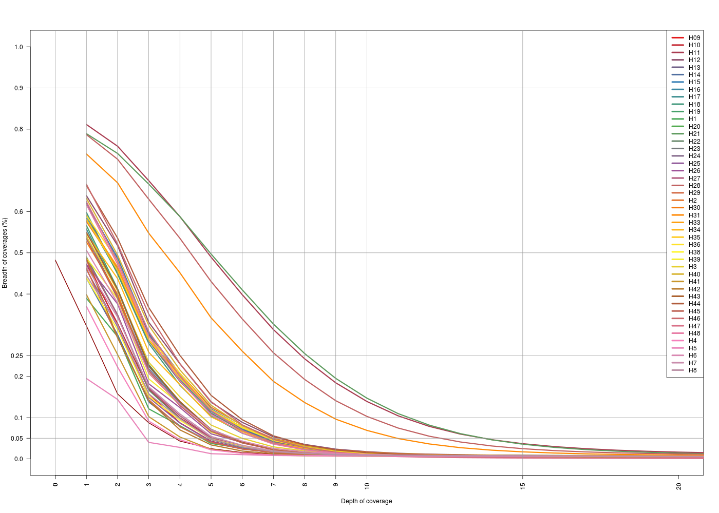 (Click image to enlarge) (Click image to enlarge) |
 (Click image to enlarge) (Click image to enlarge) |
| X-axis: 0-20 | X-axis: 0-20 |
- For the
map2Annadataset, for both off-target sets breadth vs. depth looks the same. Same situation with themat2Swiftdataset. - For the
map2Anna, we see that the general depth is low, 25% of the off-target regions are covered at 1x for most of the samples. - For the
map2Swift, we see that there are 3 situations:- Swift sample is the one that has more coverage in general (gray thick line)
- Anna and H10 have a “medium” level coverage
- Rest of the sample behaves in the same way as in the other dataset.
- For Anna and Swift samples makes sense that the general off-target coverage is higher because these to sample datasets come from a whole-genome sequencing (WGS) experiment.
Depth of coverage
Coverage per sample

- The 0x coverage for
AnnaBGIandSwiftBGIin themap2Annadatasets, is because these samples were not in that mapping. - It is possible to see that the general coverage of the off-target regions is < 1x for all the samples. Less than 1% of the on-target coverages seen.
Coverage per target
| Min. | 1st. Qu. | Median | Mean | 3rd. Qu | Max. | Var. | Std. Dev | |
|---|---|---|---|---|---|---|---|---|
| map2Anna | 0 | 0 | 0.002091 | 1.789 | 0.02666 | 18,010 | 5,273.295 | 72.61746 |
| map2Swift | 0 | 0 | 0.001225 | 4.87 | 0.2126 | 6,299 | 2,939.12560967077 | 54.2137031540068 |
- Most of the targets are below 1x (< 3rd.Quartile)
- The coverage among targets has a really high variability.
Relation within coverage and phylogenetic distance
I am trying to analyze if there is any correlation between the depth of coverage and the phylogenetic distance from the reference species, used for the probe generation and mapping.
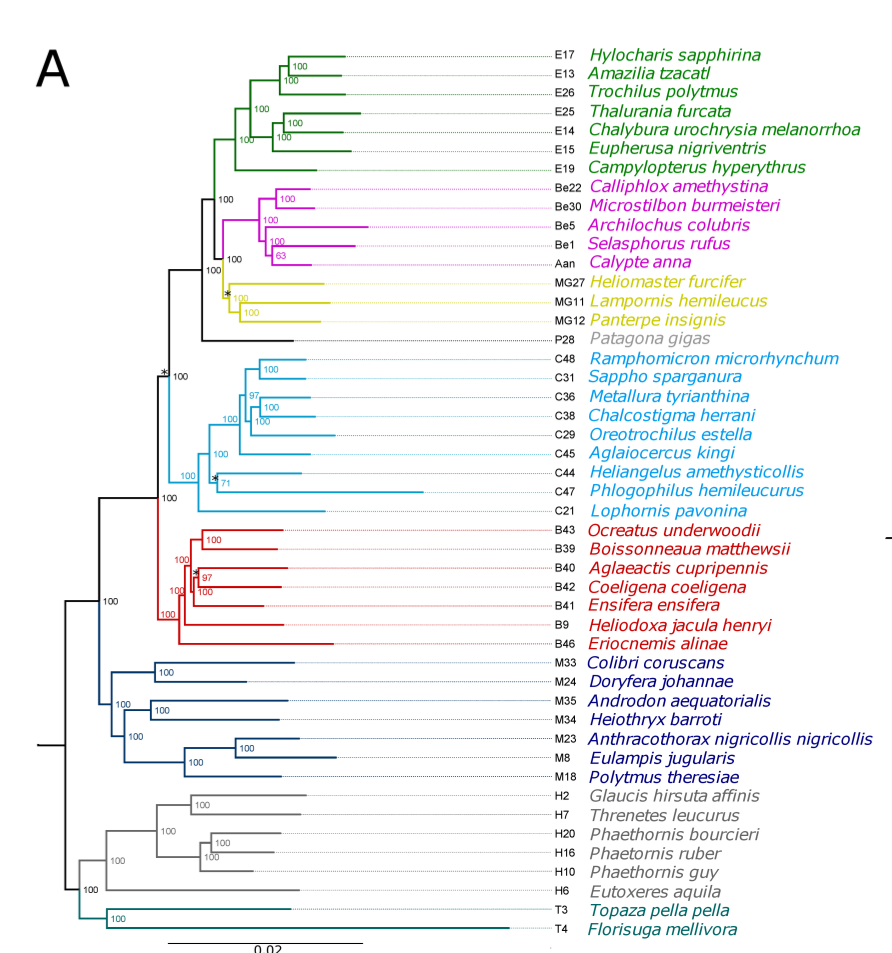
Phylogenetic reconstruction
Information of the phylogenetic reconstruction I got from the Hummingbirds Paper, this says that it was made with mitochondrial genome and nuclear gene trees using either a concatenation approach with RAxML [3] or the multi-species coalescent approach implemented in ASTRAL [4] and ASTRAL-II [5].
The phylogenies were built using subsets of the nuclear genes present the same topology between the main groups of hummingbirds with high confidence. The three subsets correspond to:
- the 2949 genes that were successfully captured (in a minimum of 8 species)
- the 1987 genes for which we could assign a high confidence swift orthologs determined in [5] (used as a root)
- the 741 genes within the latter that produced trees with average support above 50%.
This is the Supplementary Table S5 (from the Hummingbirds Paper), describing the subsets selected:
| number of genes | minimum number of sites per species (concatenated) | maximum number of sites per species (concatenated) | includes outgroup | ASTRAL score |
|---|---|---|---|---|
| 741 | 949,470 | 1,542,750 | yes | 87% |
| 1987 | 1,667,071 | 2,783,832 | yes | 78% |
| 2949 | 2,473,664 | 3,792,500 |
 (Click image to enlarge)
Cpe, outgroup reference.Aan, ingroup reference.
Depth of coverage vs. phylogenetic distance
For the analysis shown above as well as for phylogeny reconstruction using the dataset (1) with 2,949 genes.
To obtain the distance matrix I used the tree obtained with RAxML, from the concatenation of 2,750 genes. The tree gives me the branch lengths in number of substitutions per site. So, the distance calculated here, is the pairwise distance between the tips. This was done with the R package phangorn [7], and its cophenetic function. This function computes the pairwise distances between the pairs of tips from a phylogenetic network using its branch lengths.
sampleColors = colorRampPalette(brewer.pal(9, "Set1"))(48)
treefile="/home/merly/git/cph-visit/coverage-analysis/empirical/data/trees/RAxML_bipartitions.2011.concat"
tree=read.nexus(treefile)
distMatrix=cophenetic(tree)
dCpe=distMatrix["Cpe",]
dAan=distMatrix["Aan",]
distMatrix[upper.tri(distMatrix)]=NA
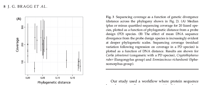
Following the figure F3A in Braggs’s paper [8], where it shows sequencing coverage as a function of genetic divergence. I have calculated the depth of coverage for both datasets and phylogenetic distance. In the plot below you can see the median target coverage per sample.

Gene-wise relation
SARA COMMENT
Is the “Detailed” part, a long description of all steps you did to get above, or different things… bit confusing to me… it seems like a different thing, where you’ll now look at this relationship PER GENE, right??
After genes with missing data were removed leaving 2,750 genes, and after matching those genes to the ones available in Swift, 1,469.
For obtain the relation between depth of coverage and phylogenetic distance gene-wise, I will used a smaller dataset (2), with 1,987 genes, which I will intersect with those from which I do have the coverage information.
To do that, I generated a new dataset from the intersection of the genes found in Calypte_anna.gene.CDS.2750.3.gff (1,469), which are those ortholog genes matching across datasets, and the available gene trees (1,988).
cat "$WD/files/Calypte_anna.gene.CDS.2750.3.gff" | cut -f9 | uniq | tr "_" " " | awk '{print $2}' | tr ";" " " > g.trees.to.filter.txt
for gtreefile in $(cat $WD/files/g.trees.to.filter.txt); do
cp "$WD/trees/gtrees/$gtreefile" "$WD/trees/gtrees.2/"
done- Gene trees not found:
R001806, R005562, R009279, R014527, R014590. - Resulting on 1,464 genes.
- Trees didn’t have branch lengths, I moved to the available multiple-sequence alignments (MSA), from which only 741 could be retrieved.
ls "$WD/trees/seqs" | tr "." " " | awk '{print $1}' > "$WD/files/g.trees.to.filter.seqs.2.txt"- From those, I generated a smaller subset of gene trees MSAs.
mkdir "$WD/trees/seqs.2"
for gtreefile in $(cat $WD/files/g.trees.to.filter.seqs.2.txt); do
filename="$WD/trees/seqs/${gtreefile}.x.aa.aln.backTranslated.gz"
cp $filename "$WD/trees/seqs.2/"
doneSARA COMMENT
You made an underlying assumption that “hamming distances” will reflect phylogenetic distance. May not be exactly like that, but, ok, I think it works to approximate.
- I calculated the pairwise distance from MSAs of the resulting gene trees, and extracted the vectors belonging to the distances to
Annaand toSwift. I did this using thedist.dna()function, from theapeRpackage, with the modelraw. This function computes a matrix of pairwise distances from DNA sequences using a model of DNA evolution. The modelrawis simply the proportion or the number of sites that differ between each pair of sequences.
geneList=unlist(read.table(paste0(WD,"g.trees.to.filter.seqs.2.txt"), stringsAsFactors=F))
distancesAnna=matrix(rep(0,length(geneList)*length(sampleNamesSwift)), length(geneList), length(sampleNamesSwift))
distancesSwift=matrix(rep(0,length(geneList)*length(sampleNamesSwift)), length(geneList), length(sampleNamesSwift))
rownames(distancesAnna)=geneList; colnames(distancesAnna)=sampleNamesSwift;
rownames(distancesSwift)=geneList; colnames(distancesSwift)=sampleNamesSwift
gtreefiles <- list.files(
path = paste0("/media/merly/Baymax/research/cph-visit/coverage-analysis/trees/seqs.2/"),
pattern="*.x.aa.aln.backTranslated")
gtreefiles=paste0("/media/merly/Baymax/research/cph-visit/coverage-analysis/trees/seqs.2/",gtreefiles)
labelsCorrect=c("H05","H01","H08","H03","H04","H06","H02","H07")
labelsWronglyFormated=c("H5","H1","H8","H3","H4","H6","H2","H7")
for (i in 1:length(gtreefiles)) {
print(i)
msa=as.matrix(read.FASTA(gzfile(gtreefiles[i])))
hammDist=as.matrix(dist.dna(msa, model="raw"))
indexAnna=which(startsWith(rownames(hammDist),"Aan"))
indexSwift=which(startsWith(rownames(hammDist),"Cpe"))
namesIds=which(rownames(hammDist) %in% labelsCorrect)
rownames(hammDist)[c(indexAnna, indexSwift, namesIds)]=c("AnnaBGI","SwiftBGI",labelsWronglyFormated)
colnames(hammDist)[c(indexAnna, indexSwift, namesIds)]=c("AnnaBGI","SwiftBGI",labelsWronglyFormated)
gene=strsplit(basename(gtreefiles[i]),"\\.")[[1]][1]
distancesAnna[gene,colnames(distancesAnna)]=hammDist[indexAnna,colnames(distancesAnna)]
distancesSwift[gene,colnames(distancesSwift)]=hammDist[indexSwift,colnames(distancesSwift)]
}
write.table(distancesAnna,file=paste0(WD,"distance.matrix.per.gene.anna.txt"), col.names=T,row.names=T)
write.table(distancesSwift,file=paste0(WD,"distance.matrix.per.gene.swift.txt"), col.names=T,row.names=T)- Afterwards, I filtered them to match those genes from which coverage was calculated. Leaving a total of 623 genes to work with.
distancesAnna=read.table(file=paste0(WD,"distance.matrix.per.gene.anna.txt"), header=T)
distancesSwift=read.table(file=paste0(WD,"distance.matrix.per.gene.swift.txt"), header=T)
birds48filename=paste0(WD,"48birds_ortholog.list.chi.anna.cpe.hum.finch")
birds=read.table(birds48filename, header=T,
colClasses=c("character","numeric","character","character",
"character","character","character"))
birds.2=birds[birds$anna!="-",]
birds.3=birds.2[birds.2$swift!="-",]
birds.4=unique(birds.3)
birds.5=birds.4[,c("anna","swift")]
birds.5$swift=paste0("Parent=",birds.5$swift,";")
birds.5$anna=paste0("Parent=Aan_", birds.5$anna,";")
annaGenes=unique(gffAnna$V9)
birds.6=birds.5[birds.5$anna %in% annaGenes, ]
birds.6$swift.plain=unlist(strsplit(unlist(lapply(strsplit(birds.6$swift,"_"), function(x){x[[2]]})), ";"))
birds.6$anna.plain=unlist(strsplit(unlist(lapply(strsplit(birds.6$anna,"_"), function(x){x[[2]]})), ";"))
smallbird=birds.6[birds.6$anna.plain %in% intersect(birgit status
ds.6$anna.plain,geneList),]
distancesAnna=distancesAnna[smallbird$anna.plain,]
distancesSwift=distancesSwift[smallbird$anna.plain,]
rownames(distancesAnna)=smallbird$anna
rownames(distancesSwift)=smallbird$swift- Retrieved the coverage information per gene and filtered the coverage matrices to match the 623 resulting genes.
samplesFilenameAnna="/home/merly/git/cph-visit/coverage-analysis/empirical/data/anna/samples.txt"
samplesFilenameSwift="/home/merly/git/cph-visit/coverage-analysis/empirical/data/swift/samples.txt"
sampleNamesAnna=unlist(read.table(samplesFilenameAnna, stringsAsFactors = F))
sampleNamesSwift=unlist(read.table(samplesFilenameSwift, stringsAsFactors = F))
coverageMatrixFileAnna="/home/merly/git/cph-visit/coverage-analysis/empirical/data/anna/coverage.matrix.per.gene.txt"
coverageMatrixFileSwift="/home/merly/git/cph-visit/coverage-analysis/empirical/data/swift/coverage.matrix.per.gene.txt"
coverageMatrixAnna=read.table(coverageMatrixFileAnna, header=T)/genesAnna$Size
coverageMatrixSwift=read.table(coverageMatrixFileSwift, header=T)/genesSwift$Size
rownames(coverageMatrixAnna)=genesAnna$Gene
rownames(coverageMatrixSwift)=genesSwift$Gene
#-------------------------------------------------------------------------------
cmswift=coverageMatrixSwift[smallbird$swift,]
cmanna=coverageMatrixAnna[smallbird$anna,]
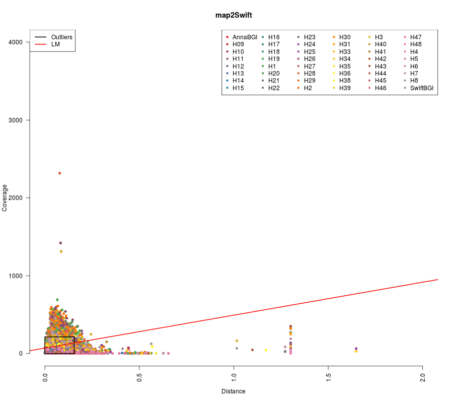
cmanna=cbind(cmanna,AnnaBGI=rep(0,nrow(cmanna)), SwiftBGI=rep(0,nrow(cmanna)))- Linear correlation was calculated after removing outliers in both coverage and distance
- What is shown in the plot below is the relation between depth of coverage and phylogenetic distance per gene per sample. 623 genes were used. 48 Samples.
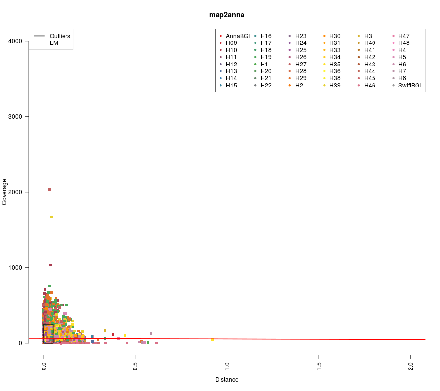
(Click image to enlarge)
##
## Call:
## lm(formula = finalCoverageSwift ~ finalDistanceSwift)
##
## Residuals:
## Min 1Q Median 3Q Max
## -62.29 -36.23 -12.25 23.84 152.52
##
## Coefficients:
## Estimate Std. Error t value Pr(>|t|)
## (Intercept) 62.9422 0.8903 70.696 <2e-16 ***
## finalDistanceSwift -8.1952 11.2783 -0.727 0.467
## ---
## Signif. codes: 0 ‘***’ 0.001 ‘**’ 0.01 ‘*’ 0.05 ‘.’ 0.1 ‘ ’ 1
##
## Residual standard error: 48.22 on 20806 degrees of freedom
## Multiple R-squared: 2.538e-05, Adjusted R-squared: -2.269e-05
## F-statistic: 0.528 on 1 and 20806 DF, p-value: 0.4675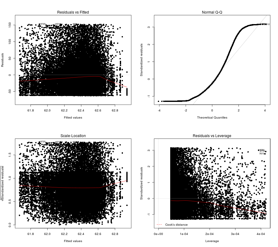
(Click image to enlarge)
(Click image to enlarge)
##
## Call:
## lm(formula = finalCoverageAnna ~ finalDistanceAnna)
##
## Residuals:
## Min 1Q Median 3Q Max
## -91.18 -39.74 -12.89 26.50 182.16
##
## Coefficients:
## Estimate Std. Error t value Pr(>|t|)
## (Intercept) 70.0355 0.6766 103.52 <2e-16 ***
## finalDistanceAnna 423.2795 33.4987 12.64 <2e-16 ***
## ---
## Signif. codes: 0 ‘***’ 0.001 ‘**’ 0.01 ‘*’ 0.05 ‘.’ 0.1 ‘ ’ 1
##
## Residual standard error: 54.82 on 19718 degrees of freedom
## Multiple R-squared: 0.008032, Adjusted R-squared: 0.007982
## F-statistic: 159.7 on 1 and 19718 DF, p-value: < 2.2e-16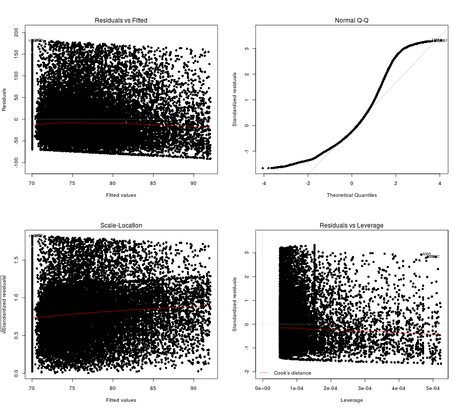
(Click image to enlarge)
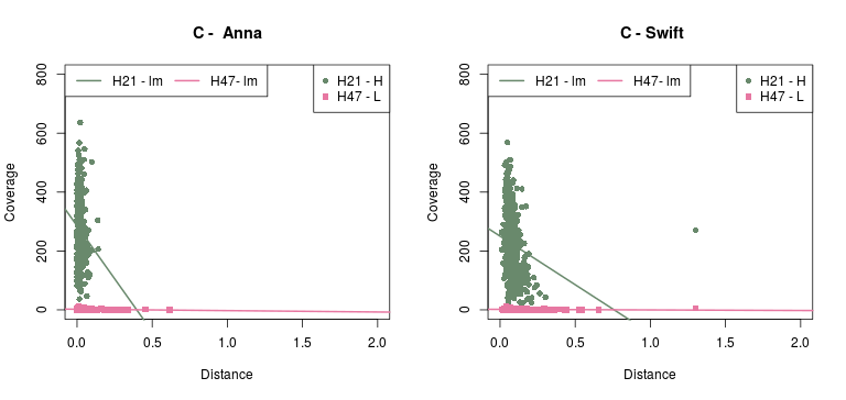
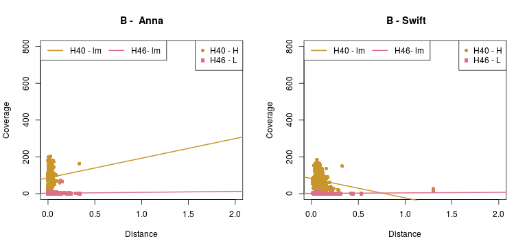
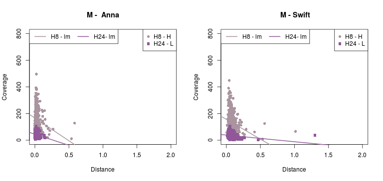
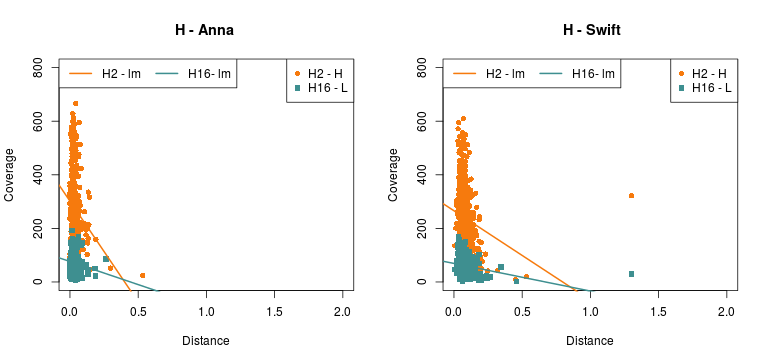
Detailed - pairs per species
Now, the plots below show the relation between phylogenetic distance and coverage, of two (2) samples from the Cocquettes, Brilliants, Mangoes and Hermits groups, following the ML tree from the Hummingbird paper (F1,A). These samples correspond to one with high coverage and one with low coverage.
(Click image to enlarge)
(Click image to enlarge)
(Click image to enlarge)
(Click image to enlarge)
(Click image to enlarge)
(Click image to enlarge)
P - values
| Coquettes | Brilliants | Mangoes | Hermits | |
|---|---|---|---|---|
| Low Coverage - map2Anna | 0.0078472 | 0.1558059 | 1.52e-05 | 0.0000023 |
| High Coverage - map2Anna | 0.0000386 | 0.1587529 | 1.43e-04 | 0.0054126 |
| Low Coverage - map2Swift | 0.0000003 | 0.0000021 | 0.00e+00 | 0.0000091 |
| High Coverage - map2Swift | 0.0031817 | 0.0045679 | 8.60e-06 | 0.0000005 |
Summary
- Important features of this report are the coverage distributions per individual/gene/target.
- For individual coverage distribution, it looks like a bimodal distribution, but I have no knowledge on how of parameterize this distribution.
- I simulated the discussed (in April) coverage distribution for individuals, and here can be found the described scenarios:
- Scenario 1: alpha shape from LN:1.2,1 (http://merly.escalona.com.es/research/phd/reports/cph-visit/coverage.parameterization.LN1.2-1.html)
- Scenario 2: alpha shape from LN:1.4,1 (http://merly.escalona.com.es/research/phd/reports/cph-visit/coverage.parameterization.LN1.4-1.html)
- Scenario 3: alpha shape from LN:1.5,1 (http://merly.escalona.com.es/research/phd/reports/cph-visit/coverage.parameterization.LN1.5-1.html)
- I simulated the discussed (in April) coverage distribution for individuals, and here can be found the described scenarios:
- As for the loci coverage distribution, they can follow either a Poisson or also a Gamma distribution, I guess this depends on what we are going to call a “locus”, if it is more a gene-like or a target-like definition.
- Considering loci as genes, coverage distribution should then follow a Poisson, mean
100and standard deviation~40 - Considering targets of this experiment, coverage distribution can then be simulated with the Gamma-based multiplier already agreed for the individual coverage variation..
- Considering loci as genes, coverage distribution should then follow a Poisson, mean
- Percentage of targets not captured is
~2%which for this case is not known if it is just because of the capture, or if it is because some of the targets used for mapping were not used to design the probes. - The on/off target coverage variation:
- Taking into account the coverage of the on-target regions for this data (mean
~100x), the off-target regions have less that 1% of the mean coverage, and so I think that the variation predicted fits perfectly.
- Taking into account the coverage of the on-target regions for this data (mean
- Phylogenetic coverage decay:
- For the analysis made with the concatenated tree in RaxML, results seem consistent with that found in the Bragg et al. paper.

- As for the information in the Detailed - pairs per species, since it is difficult to see any correlation with the previous data, Rute suggested to check out the gene-coverage relation. So I took 2 individuals from 4 main species which distance to the reference increases from Coquettes towards Hermits (can be seen in the tree from the paper above). These individual where selected by their coverage, getting a high and a low coverage patterns so it could be easier to see if there was any correlation.
- Disclaimers:
- The method used for the calculation of the phylogenetic distance may not be the proper one.
- I’m not completely confident that the correlation was computed correctly.
- From these I can only take into consideration the p-values from the linear model fitting, which do not say for all that the existence of a linear correlation is statistically significant.
- Disclaimers:
- For the analysis made with the concatenated tree in RaxML, results seem consistent with that found in the Bragg et al. paper.
Source files
Bash script with the commands for the coverage calculation [bash] Download
On target coverage analysis [Rscript] Download
Off target coverage analysis [Rscript] Download
Phylogenetic distance vs. depth of coverage (Gene-wise) Download
Phylogenetic distance vs. depth of coverage (RaxML) Download
References
- [1] Gilbert, M, P; Jarvis, E, D; Li, B; Li, C; Mello, C, V; The Avian Genome Consortium, ; Wang, J; Zhang, G (2014): Genomic data of the Anna’s Hummingbird (Calypte anna). GigaScience Database. DOI: 10.5524/101004
- [2] Gilbert, M, P; Jarvis, E, D; Li, B; Li, C; The Avian Genome Consortium, ; Wang, J; Zhang, G (2014): Genomic data of the Chimney Swift (Chaetura pelagica). GigaScience Database. DOI: 10.5524/101005
- [3]: Bleiweiss R, Kirsch JAW, Matheus JC (1994) DNA-DNA Hybridization Evidence for Sub-family Structure among Hummingbirds. Auk 111(1):8–19. DOI: 10.2307/4088500
- [4]: McGuire JA, et al. (2014) Molecular phylogenetics and the diversification of hummingbirds. Curr Biol 24(8):910–6. DOI: 10.1016/j.cub.2014.03.016
- [5]: Stamatakis A (2014) RAxML version 8: a tool for phylogenetic analysis and post-analysis of large phylogenies. Bioinformatics 30(9):1312–1313. DOI: 10.1093/bioinformatics/btu033
- [6]: Mirarab S, et al. (2014) ASTRAL: genome-scale coalescent-based species tree estimation. Bioinformatics 30(17):i541–8. DOI: 10.1093/bioinformatics/btu462
- [7]: Mirarab S, Warnow T (2015) ASTRAL-II: coalescent-based species tree estimation with many hundreds of taxa and thousands of genes. Bioinformatics 31(12):i44–52. DOI: 10.1093/bioinformatics/btv234
- [8]: Jarvis ED, et al. (2014) Whole Genome Analyses Resolve the Early Branches in the Tree of Life of Modern Birds. Science (80- ) 346(6215):1320–1331. DOI: 10.1126/science.1253451
- [9]: Klaus Peter Schliep (2011) phangorn: phylogenetic analysis in R. Bioinformatics 27 (4): 592-593. DOI: 10.1093/bioinformatics/btq706
- [10]: Bragg, JG., Potter, S., Bi. K. and Moritz, C. (2016) Exon capture phylogenomics: efficacy across scales of divergence Molecular Ecology Resources 16, 1059–1068. DOI: 10.1111/1755-0998.12449
- [22] Aaron R. Quinlan Ira M. Hall (2010) BEDTools: a flexible suite of utilities for comparing genomic features Bioinformatics 26 (6): 841-842. DOI: 10.1093/bioinformatics/btq033
- [10] Korneliussen, Thorfinn S. and Albrechtsen, Anders and Nielsen, Rasmus (2014) ANGSD: Analysis of Next Generation Sequencing Data BMC Bioinformatics 15:356. DOI: 10.1186/s12859-014-0356-4